Data & AI · · 9 min read
Differential Evolution, Live
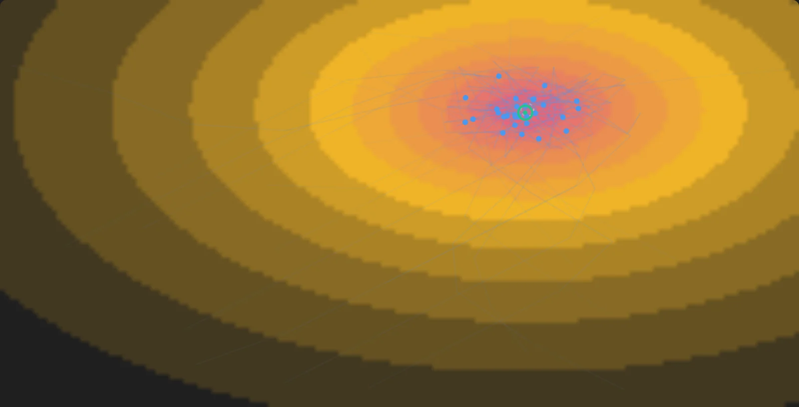
Differential evolution running live in your browser: a population whose own spread sets its step size hunts minima on four landscapes.
Differential Evolution, Live
This is part seven of the Algorithms, Live series. So far:
- ants have foraged
- triangles have evolved
- a search has cooled its way out of bad valleys
- a swarm has chased its own best guess
- a stuck search has widened its neighbourhood until it came unstuck
- a cloud of samples has learned the shape of a valley
Today's algorithm is for hard continuous problems: differential evolution. It's one of the simpler of the evolutionary family, a few lines of arithmetic wrapped in a loop. I was first properly introduced to it by Prof. Cedric Gondro, at Michigan State University, as it's one of his favorite algorithms, so we were considering its use for genomic prediction problems.
Quick jargon guide
- Differential evolution (DE): an optimiser that improves a population of candidate points by adding scaled differences between population members to other members, keeping each change only if it scores better.
- Difference vector: the arrow from one population member to another (\(b - c\)). It encodes a direction and a distance the population currently spans, and it is the raw material every DE move is built from.
- Mutant / donor vector: the new candidate built by adding a scaled difference vector to a third member: \(a + F(b - c).\) Also called the donor, because it donates coordinates during crossover.
- Crossover rate (CR): the probability that each coordinate of the trial point is taken from the mutant rather than from the parent. High \(\mathit{CR}\) means big coordinated moves. Low \(\mathit{CR}\) means one-coordinate-at-a-time nudges.
- Scale factor (F): the multiplier on the difference vector. It scales the population's own geometry up or down but never replaces it.
- Premature convergence: the population huddling into one small region before it has found the best basin. In DE this is doubly fatal, because a huddled population can only generate tiny difference vectors, so it loses the ability to leave.
Subtraction as a search strategy
Here is DE/rand/1/bin[1]: keep a population of points scattered over the landscape. To improve any one of them:
- Pick three other members at random: \(a\), \(b\), and \(c\).
- Build a mutant: take the difference vector from \(c\) to \(b\), scale it by \(F\), and add it to \(a\). In symbols, \(a + F(b - c).\)
- Crossover: build a trial point by taking each coordinate from the mutant with probability \(\mathit{CR}\), otherwise keeping the parent's coordinate. (One coordinate is always taken from the mutant, so the trial is never a clone of the parent.)
- Greedy selection: score the trial. If it beats the parent, it takes the parent's seat in the population. If not, it is thrown away and the parent stays.
Do that once for every member to create a generation. Repeat!
Every other optimiser in this series had to decide how big a move to make: simulated annealing had a cooling schedule, the genetic algorithm had a mutation rate, gradient descent has a learning rate. DE samples a difference between two of its own members and uses that as the move.
Early in a run the population is sprayed across the whole landscape, so the differences are long and the moves are large. As the population drains into a valley, its members bunch together, the differences between them shrink, and the move size shrinks too.
The difference vectors shrink, and they also point somewhere useful. If the population has settled along a curved valley, the differences between members mostly run along that valley, so mutants get launched along it too.
The population becomes a rough map of the terrain it's sitting on. The state you already have to keep doubles as the search geometry.
Watch the geometry
You probably get this now if you're reading through the series, but here goes: the demo below runs DE on a choice of four classic test landscapes. The coloured ground is the fitness surface (deeper blue is worse, the ground fades toward the background where it is low, and a small cross marks the global minimum). The blue dots are the population, and the green ring is the best point found so far.
Each generation, one member of the population gets its donor construction drawn in full: the three amber dots are \(a\), \(b\), and \(c\), the dashed amber arrow is the difference vector from \(c\) to \(b\), and the red arrow is that same vector scaled by \(F\) and grafted onto \(a\), ending at the mutant (the hollow red circle). The red diamond is the trial point after crossover, ringed if it won its duel with the parent.
Then compare the arrows at generation two with the arrows at generation sixty. Same code, same \(F\), and the moves have shrunk by orders of magnitude because the population did.
Click (or tap) anywhere on the landscape to re-seed the whole population as a tight cluster around that spot and watch it fan out or slide home.
Spread is the mean distance from each member to the population's centre. Mean step is the average length of \(F(b - c)\) this generation. Both charts use log scales, so self-scaling convergence shows up as a roughly straight downhill line. On the Egg carton, watch the population straddle several dimples before it commits. On the Banana valley, watch the difference vectors line up with the curve of the valley floor.
F, CR, and a population of eight
Drop \(\boldsymbol{F}\) to 0.1 on the Egg carton. Every move is now a tenth of a population difference, so members can only creep to the nearest dimple. The spread collapses early, usually before anyone has found the central basin.
Then the trap springs. A huddled population can only make tiny difference vectors, so the step size follows the spread down and the search is welded shut. Self-scaling, run in reverse. The best-fitness line goes flat while the spread line dives, and that is premature convergence.
Now push \(\boldsymbol{F}\) to 1.8. Every mutant overshoots the region the population spans, so the population becomes a spray. The spread line stops falling, the mean step stays huge, and best fitness improves only by luck. DE needs the population to contract for its thermometer to read cooler. At \(F\) this high, contraction never begins.
Set \(\boldsymbol{\mathit{CR}}\) near zero on the Banana valley. Each trial now differs from its parent in a single coordinate, so the search moves like a rook: horizontally or vertically, never diagonally. The banana valley is curved, and progress along it needs both coordinates to change together.
Watch the population inch along in tiny axis-aligned stair steps. Then push \(\mathit{CR}\) back up to 0.9 and watch it slide along the valley in coordinated diagonal moves. \(\mathit{CR}\) is the knob that decides whether DE moves one coordinate at a time or as whole vectors.
Shrink the population to 8. The difference vectors are now drawn from a pool of a few dozen possible pairs, so the same handful of directions gets recycled over and over.
Diversity is essential and a tiny population runs out of it almost immediately: fast convergence, frequently to the wrong dimple. The genetic algorithm in part two had the same failure for the same reason, a gene pool too small to explore with.
The missing knob
Put this next to the genetic algorithm from part two and the family resemblance is obvious: a population, mutation, crossover, selection. The GA shuffled bits and letters. DE does arithmetic on real vectors. The GA made mutation from coin flips and a fixed rate you had to tune. DE makes mutation out of the population itself, so the operator adapts as the population does.
And the GA ran a selection lottery where fit parents got more tickets. DE holds one duel per seat, child against its own parent, winner sits. The best member can only be replaced by something better.
Its sophisticated cousin CMA-ES learns an explicit statistical model of where good moves live and updates it with some fairly serious mathematics. DE gets a decent share of the same benefit, steps that stretch along the good directions and shrink as the search closes in, using subtraction.
It is dumber than CMA-ES generally, but very much stands on its own, regardless!
Where DE turns up in practice
Storn and Price introduced it in 1997[1], it won early optimisation competitions, and it is still a default first try in engineering optimisation: antenna design, power systems, chemical process tuning, anywhere someone has a black-box simulator with a dozen real-valued dials. The survey literature on its variants runs to hundreds of papers[2].
You can buy adaptivity: learned models, schedules, meta-parameters. Or you can arrange the algorithm so the state it already keeps is the adaptation. DE gets self-scaling search out of a subtraction.
Go and set the Egg carton running, click somewhere daft to strand the population in a corner, and watch the arrows do the rest.
Common questions
Why is it called "differential" evolution?
For the difference vectors: every mutation is built from the difference between two population members. It has nothing to do with differential equations or with derivatives.
How do I pick F and CR in practice?
The folklore defaults hold up surprisingly well: \(F\) between 0.5 and 0.9, \(\mathit{CR}\) around 0.9. This demo starts at \(F = 0.8\), \(\mathit{CR} = 0.9\). Low \(\mathit{CR}\) only helps when your variables are independent of each other, which you rarely know in advance, so high \(\mathit{CR}\) is the safer bet. If you'd rather not choose at all, self-adaptive variants such as jDE and SaDE evolve \(F\) and \(\mathit{CR}\) alongside the solutions, and the Das and Suganthan survey covers them at length[2].
Doesn't greedy selection cause the premature convergence you just demonstrated?
Less than you'd think. The duel is greedy about who survives, but the moves themselves come from the whole population's geometry, and that keeps exploration alive as long as the population is spread out. What kills the search in the \(F = 0.1\) experiment is the spread collapsing before the good basin is found. Greedy replacement plus population-shaped mutation is a surprisingly stable pairing, and it's a big part of why DE needs so little babysitting.
References
- Storn, R., & Price, K. (1997). Differential Evolution - A Simple and Efficient Heuristic for global Optimization over Continuous Spaces. Journal of Global Optimization, 11(4), 341–359. https://doi.org/10.1023/A:1008202821328
- Das, S., & Suganthan, P. N. (2011). Differential Evolution: A Survey of the State-of-the-Art. IEEE Transactions on Evolutionary Computation, 15(1), 4–31. https://doi.org/10.1109/TEVC.2010.2059031